R语言：多元线性回归和模型检验

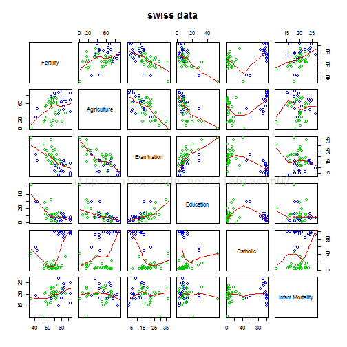
利用swiss数据集进行多元线性回归研究

# 先查看各变量间的散点图　　

pairs(swiss, panel = panel.smooth, main = "swiss data",

col = 3 + (swiss$Catholic > 50))

# 利用全部变量建立多元线性回

a=lm(Fertility ~ . , data = swiss)

summary(a)

##

## Call:

## lm(formula = Fertility ~ ., data = swiss)

##

## Residuals:

## Min 1Q Median 3Q Max

## -15.274 -5.262 0.503 4.120 15.321

##

## Coefficients:

## Estimate Std. Error t value Pr(>|t|)

## (Intercept) 66.9152 10.7060 6.25 1.9e-07 ***

## Agriculture -0.1721 0.0703 -2.45 0.0187 *

## Examination -0.2580 0.2539 -1.02 0.3155

## Education -0.8709 0.1830 -4.76 2.4e-05 ***

## Catholic 0.1041 0.0353 2.95 0.0052 **

## Infant.Mortality 1.0770 0.3817 2.82 0.0073 **

## ---

## Signif. codes: 0 "***" 0.001 "**" 0.01 "*" 0.05 "." 0.1 " " 1

##

## Residual standard error: 7.17 on 41 degrees of freedom

## Multiple R-squared: 0.707, Adjusted R-squared: 0.671

## F-statistic: 19.8 on 5 and 41 DF, p-value: 5.59e-10

# 从结果看，Education变量的ｐ值一颗星就都没有，说明对模型极不显著。

# R中提供了add1 drop1函数来针对线性模型进行变量的增减处理

drop1(a)

## Single term deletions

##

## Model:

## Fertility ~ Agriculture + Examination + Education + Catholic +

## Infant.Mortality

## Df Sum of Sq RSS AIC

## <none> 2105 191

## Agriculture 1 308 2413 195

## Examination 1 53 2158 190

## Education 1 1163 3268 209

## Catholic 1 448 2553 198

## Infant.Mortality 1 409 2514 197

# 从结果看，去掉Education这个变量后，AIC最小，所以下一步可以剔除该变量进行建模。

b=update(a,.~.-Education)

summary(b)

##

## Call:

## lm(formula = Fertility ~ Agriculture + Examination + Catholic +

## Infant.Mortality, data = swiss)

##

## Residuals:

## Min 1Q Median 3Q Max

## -23.919 -3.553 -0.649 6.596 14.177

##

## Coefficients:

## Estimate Std. Error t value Pr(>|t|)

## (Intercept) 59.6027 13.0425 4.57 4.2e-05 ***

## Agriculture -0.0476 0.0803 -0.59 0.55669

## Examination -0.9680 0.2528 -3.83 0.00042 ***

## Catholic 0.0261 0.0384 0.68 0.50055

## Infant.Mortality 1.3960 0.4626 3.02 0.00431 **

## ---

## Signif. codes: 0 "***" 0.001 "**" 0.01 "*" 0.05 "." 0.1 " " 1

##

## Residual standard error: 8.82 on 42 degrees of freedom

## Multiple R-squared: 0.545, Adjusted R-squared: 0.501

## F-statistic: 12.6 on 4 and 42 DF, p-value: 8.27e-07

#从接下来的结果看，有两个变量不显著，Ｒ平方也仅有0.53，模型效果极不理想。需要进一步进行研究。

# 幸好Ｒ有step函数，可以对模型进行变量自动筛选，根据AIC最小原则进行

b=step(a,direction="backward")

## Start: AIC=190.7

## Fertility ~ Agriculture + Examination + Education + Catholic +

## Infant.Mortality

##

## Df Sum of Sq RSS AIC

## - Examination 1 53 2158 190

## <none> 2105 191

## - Agriculture 1 308 2413 195

## - Infant.Mortality 1 409 2514 197

## - Catholic 1 448 2553 198

## - Education 1 1163 3268 209

##

## Step: AIC=189.9

## Fertility ~ Agriculture + Education + Catholic + Infant.Mortality

##

## Df Sum of Sq RSS AIC

## <none> 2158 190

## - Agriculture 1 264 2422 193

## - Infant.Mortality 1 410 2568 196

## - Catholic 1 957 3115 205

## - Education 1 2250 4408 221

summary(b)

##

## Call:

## lm(formula = Fertility ~ Agriculture + Education + Catholic +

## Infant.Mortality, data = swiss)

##

## Residuals:

## Min 1Q Median 3Q Max

## -14.676 -6.052 0.751 3.166 16.142

##

## Coefficients:

## Estimate Std. Error t value Pr(>|t|)

## (Intercept) 62.1013 9.6049 6.47 8.5e-08 ***

## Agriculture -0.1546 0.0682 -2.27 0.0286 *

## Education -0.9803 0.1481 -6.62 5.1e-08 ***

## Catholic 0.1247 0.0289 4.31 9.5e-05 ***

## Infant.Mortality 1.0784 0.3819 2.82 0.0072 **

## ---

## Signif. codes: 0 "***" 0.001 "**" 0.01 "*" 0.05 "." 0.1 " " 1

##

## Residual standard error: 7.17 on 42 degrees of freedom

## Multiple R-squared: 0.699, Adjusted R-squared: 0.671

## F-statistic: 24.4 on 4 and 42 DF, p-value: 1.72e-10

接下来，对建模的变量和模型进行回归诊断的研究

首先，对自变量进行正态性检验

shapiro.test(swiss$Agriculture)

##

## Shapiro-Wilk normality test

##

## data: swiss$Agriculture

## W = 0.9664, p-value = 0.193

shapiro.test(swiss$Examination)

##

## Shapiro-Wilk normality test

##

## data: swiss$Examination

## W = 0.9696, p-value = 0.2563

shapiro.test(swiss$Education)

##

## Shapiro-Wilk normality test

##

## data: swiss$Education

## W = 0.7482, p-value = 1.312e-07

shapiro.test(swiss$Catholic)

##

## Shapiro-Wilk normality test

##

## data: swiss$Catholic

## W = 0.7463, p-value = 1.205e-07

shapiro.test(swiss$Infant.Mortality)

##

## Shapiro-Wilk normality test

##

## data: swiss$Infant.Mortality

## W = 0.9776, p-value = 0.4978

对各变量的正态性检验结果来看，变量Education和Catholic的ｐ值小于0.05，故这两个变量数据不符合正态性分布。

现在，对模型的残差也进行正态性检验（回归模型的残差也要符合正态分布）

b.res<-residuals(b)

shapiro.test(b.res)

##

## Shapiro-Wilk normality test

##

## data: b.res

## W = 0.9766, p-value = 0.459

从结果来看，p值是0.459,模型残差符合正态分布

接下来，画出回归值与残差的残差图（应该符合均匀分布，即残差不管回归值如何，都具有相同分布）

par(mfrow=c(1,2))

# 画出残差图

plot(b.res~predict(b))

# 画出标准残差图

plot(rstandard(b)~predict(b))

par(mfrow=c(1,1))

从残差图来看，效果不太明显.

其实，可以直接画出残差图

par(mfrow=c(2,2))

plot(b)

par(mfrow=c(1,1))

End.

作者:谢佳标

来源:天善智能

本文均已和作者授权，如转载请与作者联系。