

逻辑回归:二分类
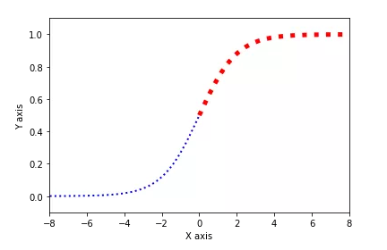
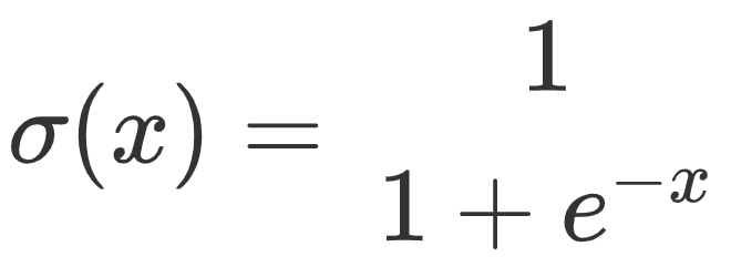
1.1 理解逻辑回归

1.2 代码实践 - 导入数据集
import numpy as npimport pandas as pdimport seaborn as snsimport matplotlib.pyplot as plt
df = pd.read_csv("https://blog.caiyongji.com/assets/hearing_test.csv")df.head()
| age | physical_score | test_result |
|
|
|
|
|
|
|
|
|
|
|
|
|
|
|
|
|
|
|
|
-
特征:1. 年龄 2. 健康得分 -
标签:(1通过/0不通过)
1.3 观察数据
sns.scatterplot(x="age",y="physical_score",data=df,hue="test_result")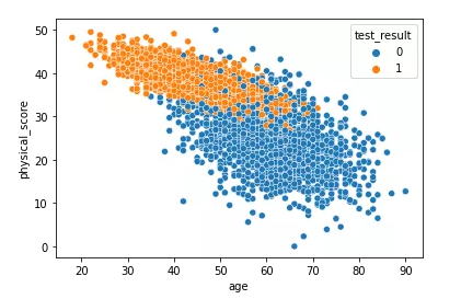
sns.pairplot(df,hue="test_result")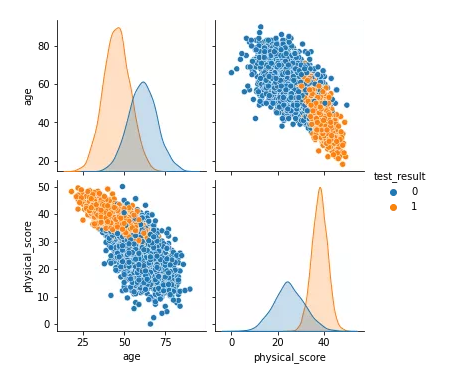
1.4 训练模型
from sklearn.model_selection import train_test_splitfrom sklearn.preprocessing import StandardScalerfrom sklearn.linear_model import LogisticRegressionfrom sklearn.metrics import accuracy_score,classification_report,plot_confusion_matrix#准备数据X = df.drop("test_result",axis=1)y = df["test_result"]X_train, X_test, y_train, y_test = train_test_split(X, y, test_size=0.1, random_state=50)scaler = StandardScaler()scaled_X_train = scaler.fit_transform(X_train)scaled_X_test = scaler.transform(X_test)#定义模型log_model = LogisticRegression()#训练模型log_model.fit(scaled_X_train,y_train)#预测数据y_pred = log_model.predict(scaled_X_test)accuracy_score(y_test,y_pred)

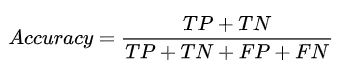
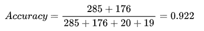
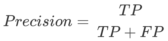
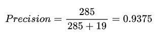
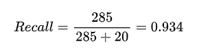
模型性能评估:准确率、精确度、召回率
plot_confusion_matrix(log_model,scaled_X_test,y_test)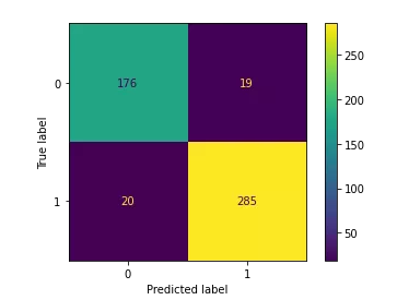
-
真正类TP(True Positive) :预测为正,实际结果为正。如,上图右下角285。 -
真负类TN(True Negative) :预测为负,实际结果为负。如,上图左上角176。 -
假正类FP(False Positive) :预测为正,实际结果为负。如,上图左下角19。 -
假负类FN(False Negative) :预测为负,实际结果为正。如,上图右上角20。

print(classification_report(y_test,y_pred))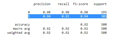

Softmax:多分类
3.1 理解 softmax 多元逻辑回归
3.2 代码实践 - 导入数据集
df = pd.read_csv("https://blog.caiyongji.com/assets/iris.csv")df.head()
| sepal_length | sepal_width | petal_length | petal_width | species |
|
|
|
|
|
|
|
|
|
|
|
|
|
|
|
|
|
|
|
|
|
|
|
|
|
|
|
|
|
|
-
特征:1. 花萼长度 2. 花萼宽度 3. 花瓣长度 4 花萼宽度 -
标签:种类:山鸢尾(setosa)、变色鸢尾(versicolor)和维吉尼亚鸢尾(virginica)
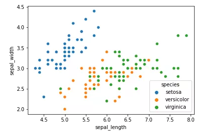
3.3 观察数据
sns.scatterplot(x="sepal_length",y="sepal_width",data=df,hue="species")我们用 seaborn 绘制花萼长度和宽度特征对应鸢尾花种类的散点图。
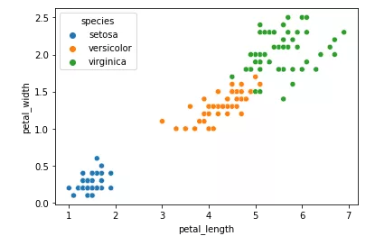
sns.scatterplot(x="petal_length",y="petal_width",data=df,hue="species")我们用 seaborn 绘制花瓣长度和宽度特征对应鸢尾花种类的散点图。
sns.pairplot(df,hue="species")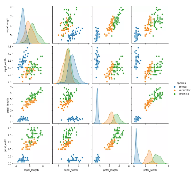
3.4 训练模型
#准备数据X = df.drop("species",axis=1)y = df["species"]X_train, X_test, y_train, y_test = train_test_split(X, y, test_size=0.25, random_state=50)scaler = StandardScaler()scaled_X_train = scaler.fit_transform(X_train)scaled_X_test = scaler.transform(X_test)#定义模型softmax_model = LogisticRegression(multi_class="multinomial",solver="lbfgs", C=10, random_state=50)#训练模型softmax_model.fit(scaled_X_train,y_train)#预测数据y_pred = softmax_model.predict(scaled_X_test)accuracy_score(y_test,y_pred)
print(classification_report(y_test,y_pred))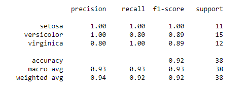
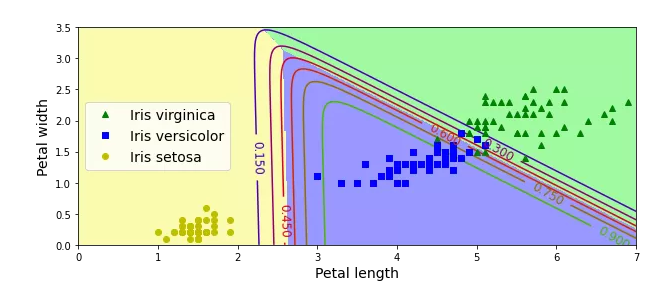
3.5 拓展:绘制花瓣分类
#提取特征X = df[["petal_length","petal_width"]].to_numpy()y = df["species"].factorize(["setosa", "versicolor","virginica"])[0]#定义模型softmax_reg = LogisticRegression(multi_class="multinomial",solver="lbfgs", C=10, random_state=50)#训练模型softmax_reg.fit(X, y)#随机测试数据x0, x1 = np.meshgrid(np.linspace(0, 8, 500).reshape(-1, 1),np.linspace(0, 3.5, 200).reshape(-1, 1),)X_new = np.c_[x0.ravel(), x1.ravel()]#预测y_proba = softmax_reg.predict_proba(X_new)y_predict = softmax_reg.predict(X_new)#绘制图像zz1 = y_proba[:, 1].reshape(x0.shape)zz = y_predict.reshape(x0.shape)plt.figure(figsize=(10, 4))plt.plot(X[y==2, 0], X[y==2, 1], "g^", label="Iris virginica")plt.plot(X[y==1, 0], X[y==1, 1], "bs", label="Iris versicolor")plt.plot(X[y==0, 0], X[y==0, 1], "yo", label="Iris setosa")from matplotlib.colors import ListedColormapcustom_cmap = ListedColormap(["#fafab0","#9898ff","#a0faa0"])plt.contourf(x0, x1, zz, cmap=custom_cmap)contour = plt.contour(x0, x1, zz1, cmap=plt.cm.brg)plt.clabel(contour, inline=1, fontsize=12)plt.xlabel("Petal length", fontsize=14)plt.ylabel("Petal width", fontsize=14)plt.legend(loc="center left", fontsize=14)plt.axis([0, 7, 0, 3.5])plt.show()

小结
-
机器学习的分类
-
机器学习的工业化流程
-
特征、标签、实例、模型的概念
-
过拟合、欠拟合
-
损失函数、最小二乘法
-
梯度下降、学习率
-
线性回归、逻辑回归、多项式回归、逐步回归、岭回归、套索(Lasso)回归、弹性网络(ElasticNet)回归是最常用的回归技术
-
Sigmoid 函数、Softmax 函数、最大似然估计
End.
作者:caiyongji
本文为转载分享,如果涉及作品、版权和其他问题,请联系我们第一时间删除(微信号:lovedata0520)
更多文章前往首页浏览http://www.itongji.cn/
- 我的微信公众号
- 微信扫一扫
-

- 我的微信公众号
- 微信扫一扫
-


评论